
KV Cache From First Principles
KV Cache explained
KV Cache
KV Caching is one of the most impactful advacements related to Large Language Models in recent times, significantly impacting both cost and latency during inference.
LLMs are autoregressive by nature—they predict each new token based on all previously attended tokens. While this approach is powerful, it creates severe inefficiencies at scale, which KV Caching addresses.
The Need for KV Caching
LLMs have a quadratic complexity O(n²), where n is the sequence length. This complexity means that the attention mechanism scales horribly with increasing sequence length. Each new token requires attending to all previous tokens, causing computational costs to grow quadratically with sequence length.
This makes LLMs highly impractical in production environments, where every millisecond of user latency and every kilobyte of GPU memory is extremely valuable. The quadratic complexity can be traced back to the attention mechanism, where much of the redundancy in matrix operations arises from the autoregressive nature of LLMs.
What happens in a decoder-only LLM
Every time inference is performed on an LLM, a prompt is provided to it in natural language. The prompt is then tokenized and broken down into a sequence of n tokens.
Based on the provided sequence of tokens, the LLM then samples the next most probable token and appends it to the initial sequence. This process continues until the LLM generates an <EOS> (End of Sequence) token, which simply means "no more text needed."
The issue is that every time a new token is generated, all the computations that were done for the previous tokens in the sequence are repeated. The way the attention mechanism works, we can easily identify this redundancy.
Lets take a look at Vanilla Attention.
(For now, kindly ignore the softmax and other operations.)
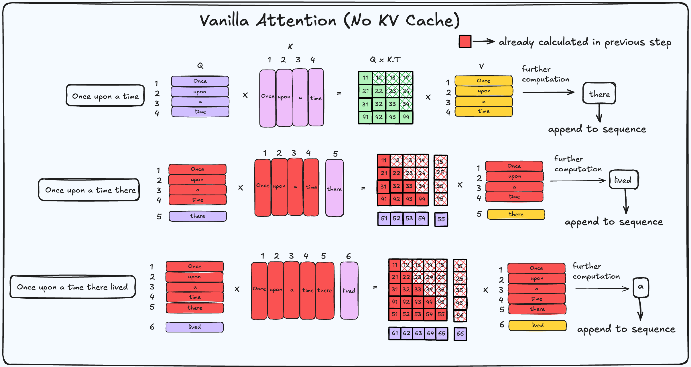
During the pre-fill stage, the whole input sequence of n tokens is passed to the LLM, and from then on, for the (n + 1)ᵗʰ token, the generation becomes autoregressive.
From the figure, we can infer that when we are generating a new token, all the required computations for the previous states have already been done. We are just wasting compute by recalculating the Query, Key, and Value matrices every single time.
Without KV Cache: Redundant Computations
| Step | Input Sequence | Keys/Values Computed | Redundant Computations |
|---|---|---|---|
| 1 | Once upon a time | K/V for "Once", "upon", "a", "time" | None |
| 2 | Once upon a time there | K/V for "Once", "upon", "a", "time", "there" | K/V recomputed for tokens 1–4 (from step 1) |
| 3 | Once upon a time there lived | K/V for "Once", "upon", "a", "time", "there", "lived" | K/V recomputed for tokens 1–5 (from steps 1–2) |
| 4 | Once upon a time there lived a | K/V for "Once", "upon", "a", "time", "there", "lived", "a" | K/V recomputed for tokens 1–6 (from steps 1–3) |
The Solution
(Spoiler Alert: KV Cache)
In computer science terms, caching refers to temporarily storing frequently accessed data in fast storage. KV Caching allows us to cache the Key and Value matrices so we need not recompute them for each sequence.
The main idea behind KV Cache is to trade off computation for memory usage because the attention mechanism is not IO aware i.e. it is more memory bound rather than compute bound. Operations in LLMs are more often bottlenecked by memory bandwidth than actual compute. By caching keys and values, we reduce redundant computations and costly memory IO operations.
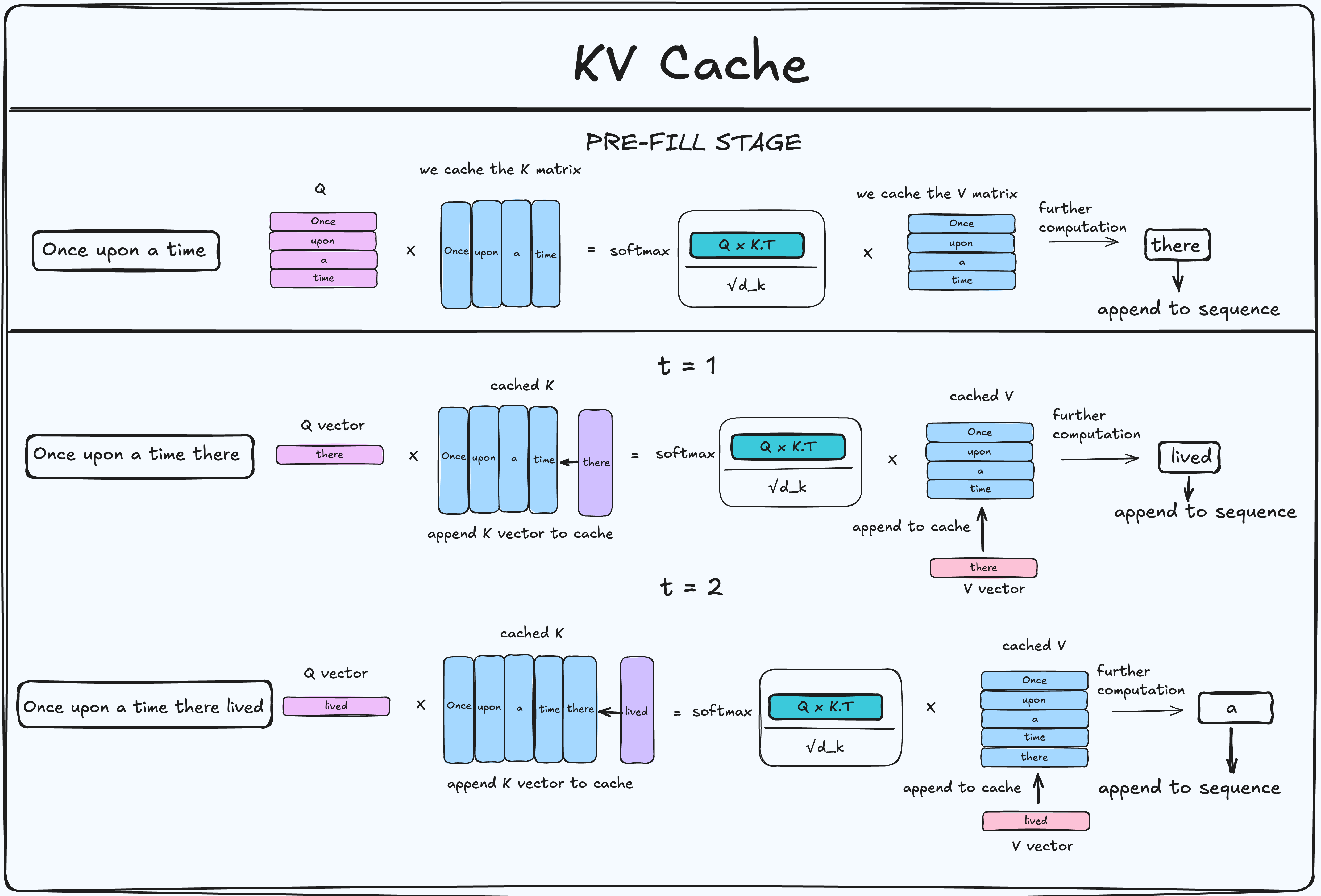
Procedure
-
Pre-fill stage
- Compute the Query, Key, and Value matrices.
- Store the Key and Value matrices as buffers (the cache).
-
Generation Stage
-
Look up the embedding for the new token.
-
Compute the Q, K, and V vectors (not full matrices).
-
Append and concatenate the new K and V vectors to the cached matrices.
-
Use only the Q vector for the new token to calculate:
-
-
Repeat this process until the
<EOS>token is generated. -
Delete the cache when a new sequence arrives to avoid providing incoherent context.
With KV Cache: No Redundant Computations
| Step | Input Sequence | Keys/Values Computed | Redundant Computations |
|---|---|---|---|
| 1 | Once upon a time | KV for tokens 1–4 | None |
| 2 | Once upon a time there | KV only for token 5 (“there”) | None |
| 3 | Once upon a time there lived | KV only for token 6 (“lived”) | None |
| 4 | Once upon a time there lived a | KV only for token 7 (“a”) | None |
Complexity
With KV caching, the time complexity reduces from O(n²) to O(n). The pre-fill phase is still O(n²), but this is a one-time cost.
KV Cache Memory Formula
For each token, the model stores Key and Value vectors for every layer and head.
- 2 → accounts for storing both K and V
- n_layers → number of transformer layers
- n_heads → number of attention heads used for KV
- d_head → dimension per head (hidden_dim ÷ n_heads)
- n_bytes → number of bytes per element (e.g., FP16 = 2, BF16 = 2, FP32 = 4)
- n_tokens → sequence length (context window)
For example:
Applying to QWEN3 0.6B
- n_layers = 28
- d_head = 64
- n_heads (KV) = 8 ← (For GQA only KV heads matter, not Q)
- n_bytes (BF16) = 2
- n_tokens = 32768
While the KV Cache consumes 1.75 GBs of memory at full context, the model parameters themselves only take about 1.4 GB. This gives us a rough idea about how at long context KV cache can also cause a memory problem.
Advantages:
- Reduced Computation: We significantly reduce the amount of computation required.
- Decreased Latency: The decreased computation also leads to lower latency and higher throughput.
Disadvantages:
- Memory Overhead: KV Cache memory size increases as the sequence length increases.
- Memory Bandwidth Bottleneck:
As the sequence length grows, the task becomes more memory-bound than compute-bound. Bandwidth refers to the transfer of weights from one memory to another. The bandwidth requirement increases with increasing sequence length.
Mitigation Strategies
- Sliding Window: Select only "m" most recent tokens from the cache to avoid bloating the context with stale tokens.
- GQA (Grouped Query Attention): Groups the KV matrices so each pair attends to multiple Query heads.
For example a common ratio of Q to KV heads is 2:1, which essentially halves the KV Cache size. - MLA (Multi-Head Latent Attention): Compresses KV matrices into a lower dimension.
DeepSeek uses this technique in their V3 model within MLA blocks where the Key and Value matrices are projected to a lower dimension. This adds a bit of compute but saves memory, providing a middle ground between compute and memory. - Quantization: Reduce memory footprint by quantizing KV matrices to lower precision (e.g., FP16 → FP8 halves memory). Accuracy may drop slightly.
- Offloading: Offload the KV Cache from GPU VRAM to system RAM or disk as sequence length grows, freeing up GPU VRAM for model and activations.
